3D
In [1]:
import numpy as np
import matplotlib.pyplot as plt
from mpl_toolkits.mplot3d import Axes3D
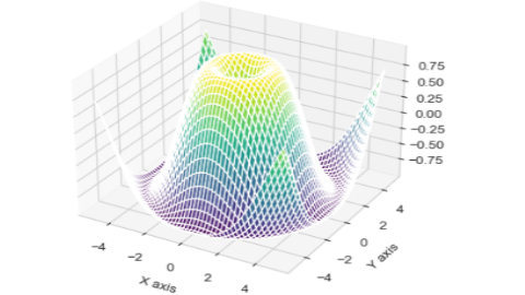
x = np.linspace(-5, 5, 100)
y = np.linspace(-5, 5, 100)
X, Y = np.meshgrid(x, y)
Z = np.sin(np.sqrt(X**2 + Y**2))
In [2]:
# plot_surface
fig = plt.figure()
ax = fig.add_subplot(111, projection='3d')
ax.plot_surface(X, Y, Z, cmap='viridis')
ax.set_xlabel('X axis')
ax.set_ylabel('Y axis')
ax.set_zlabel('Z axis')
plt.show()

In [3]:
# 3D scatter
x = np.random.standard_normal(100)
y = np.random.standard_normal(100)
z = np.random.standard_normal(100)

fig = plt.figure()
ax = fig.add_subplot(111, projection='3d')
ax.scatter(x, y, z, c='r', marker='o')
plt.show()

In [4]:
# 3D plot_wireframe
fig = plt.figure()
ax = fig.add_subplot(111, projection='3d')
ax.plot_wireframe(X, Y, Z, color='gray')
plt.show()

In [5]:
# 3D contour plot
fig = plt.figure()
ax = fig.add_subplot(111, projection='3d')
ax.contour3D(X, Y, Z, 50, cmap='binary')
plt.show()

In [6]:
import seaborn as sns
data = sns.load_dataset("mpg")
#print(data.head())

X=data['horsepower']
Y=data['weight']
Z=data['mpg']
fig = plt.figure()
ax = fig.add_subplot(111, projection='3d')
ax.scatter(X, Y, Z, c='b', marker='o')
ax.set_xlabel('horsepower')
ax.set_ylabel('weight')
ax.set_zlabel('mpg')
plt.show()
